Symmetric semi-discrete optimal transport for mesh interpolation

Agathe Herrou

sous la direction de Nicolas Bonneel, Julie Digne et Bruno Lévy

Introduction to optimal transport
Symmetric semi-discrete optimal transport
Alternating algorithm
Optimization approach
Mesh interpolation
Conclusion

Introduction to optimal transport
Symmetric semi-discrete optimal transport
Alternating algorithm
Optimization approach
Mesh interpolation
Conclusion

Optimal transport

Displacing mass under a cost minimization constraint
Canonical examples: sand piles, mines and factories

[Monge, 1781]

[Kantorovich, 1942]

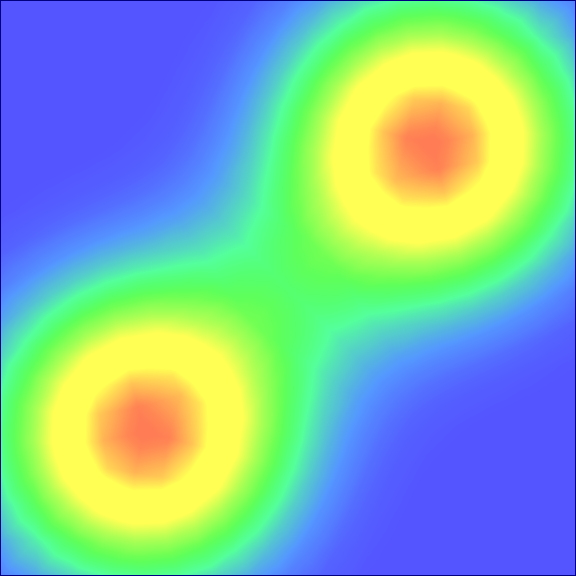
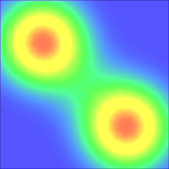
Displacement interpolation

The transport plan induces an interpolation between measures
More suited to some contexts than linear interpolation

Displacement (left) vs linear (right) interpolation

Semi-discrete optimal transport

Continuous source, discrete target

Power diagrams are equivalent to optimal transport plans [Aurenhammer et al, 1998]

Voronoi diagram: all the sites have the same influence

Limited capacities: adapt the assignment

Cell size increases as its weight decreases

Collectively adjust the weights so that the areas match the capacities

Power diagrams are equivalent to optimal transport plans [Aurenhammer et al, 1998]

Métaphore de Mérigot: boulangeries
Chaque point du domaine continu est associé à un site de l'ensemble discret.
Initialement, pain infini et boulangeries équivalentes: les gens vont à la plus proche, diagramme de Voronoi.
Si pain limité, ils changent de boulangerie si la plus proche n'a plus de pain
Changement de point de vue: plutôt que les choix des clients, on considère les prix des boulangeries. Si une boulangerie baisse ses prix il va devenir intéressant de venir de plus loin pour acheter son pain.
Si toutes les boulangeries ont des quantités de pain limitées (la même partout pour faire simple), dont la somme coïncide avec les besoins de la population, elle pourront se mettre d'accord sur les prix pour que leur clientèle corresponde exactement à leur capacité.
Cette quantité de pain produite par chaque boulangerie, c'est mathématiquement la mesure qu'on applique aux sites discrets. Dans toute la suite de l'exposé, on considérera que la mesure discrète est uniforme.
Chaque plan de transport optimal semi-discret (lorsque le coût associé est la distance au carré) peut être représenté comme un diagramme de puissance avec des poids bien choisis. Réciproquement, chaque diagramme de puissance est un plan de transport optimal pour des capacités sur les sites correspondant à l'aire de leur cellule.

Numerical computation

Cost of transporting a cell to its site

Constraint: difference between the prescribed masses and the actual masses

Weights act as Lagrange multipliers

$F$ is concave in $(\phi)$: stationary point is a maximum

Numerical algorithms

Algorithm	Author(s)	Speed	Proven convergence speed	Requirements
Gradient ascent	Aurenhammer et al, 1998	Slow	No	None
Multiscale	Mérigot, 2011	Fast	No	None
Quasi-Newton (L-BFGS)	Lévy, 2014	Fast	No	None
Newton - KMT	Kitagawa et al, 2017	Very fast	Yes	No empty cells

Alternating algorithms

Centroidal Voronoi Tessellations: Lloyd’s algorithm [Lloyd 1982, Du et al. 1999]

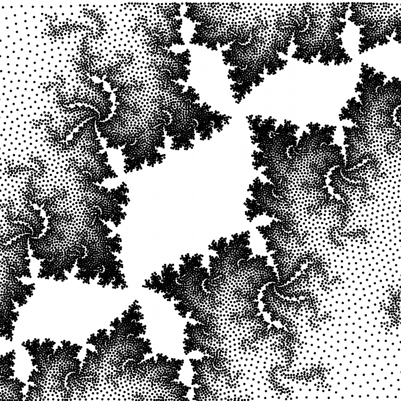
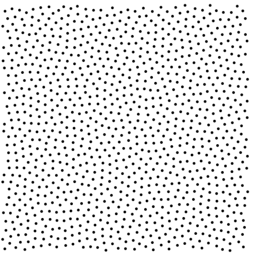
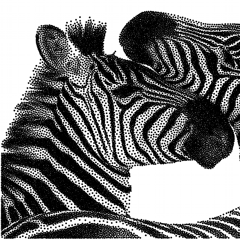
Blue Noise through Optimal Transport [de Goes et al. 2012]

Applications of semi-discrete optimal transport

Displacement interpolation [Lévy 2014]

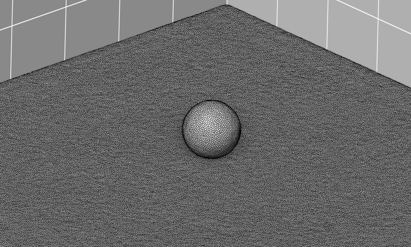
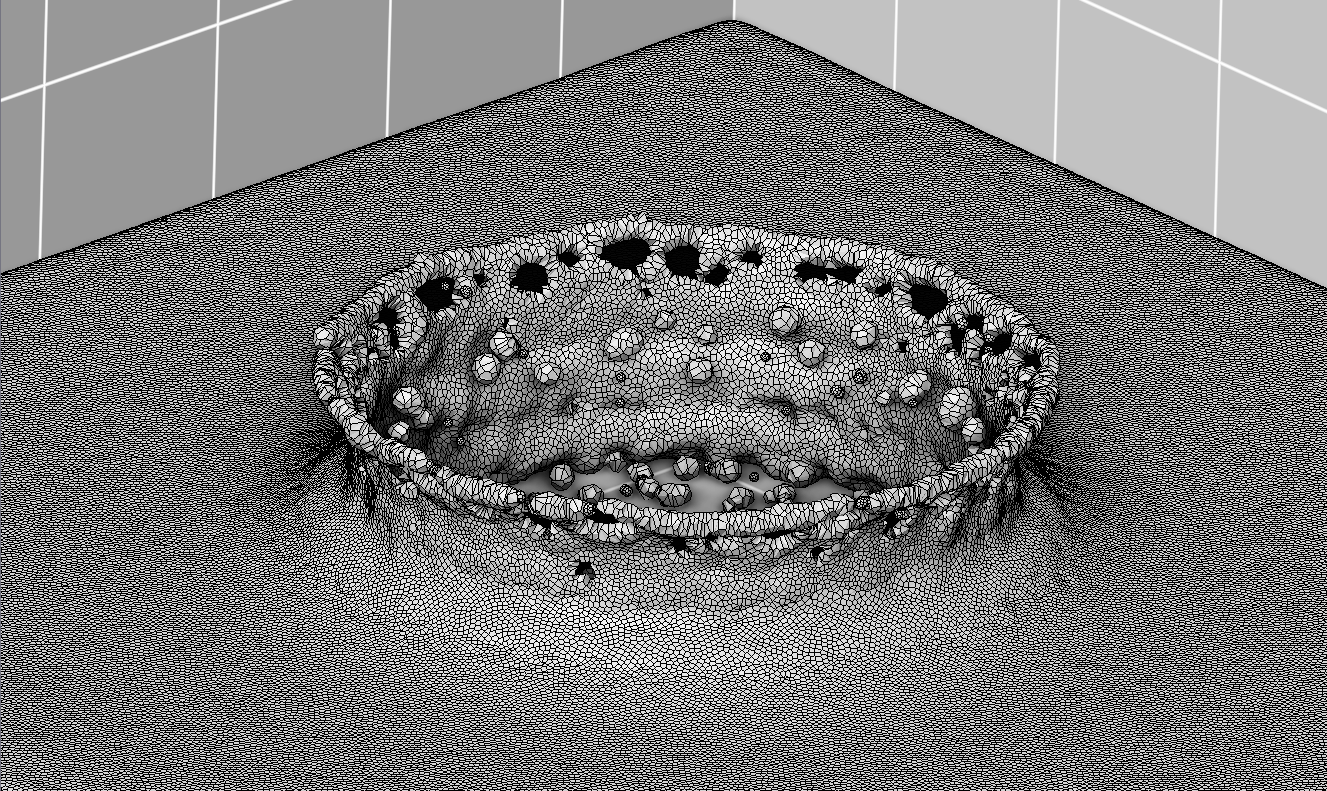
Fluid simulation [Lévy 2022]

Early universe reconstruction [Lévy et al 2021]

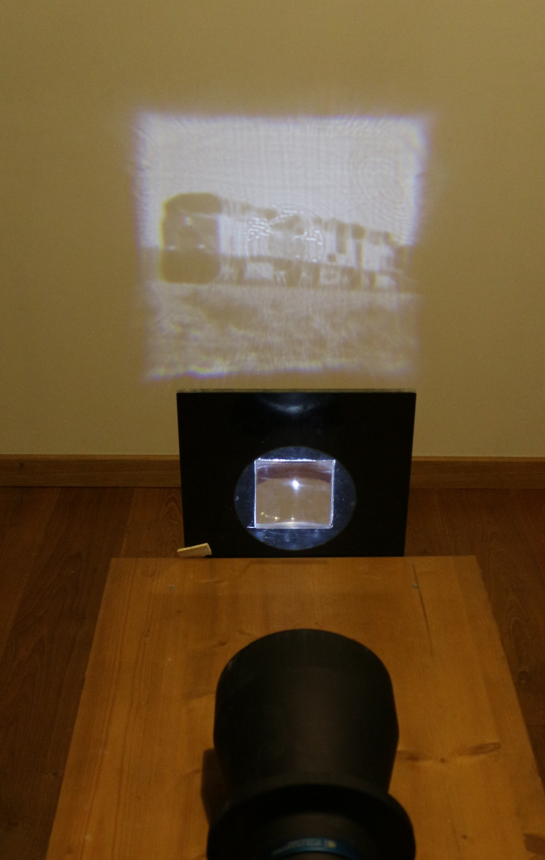
Light in Power: lenses and mirrors design [Mérigot et al 2017]

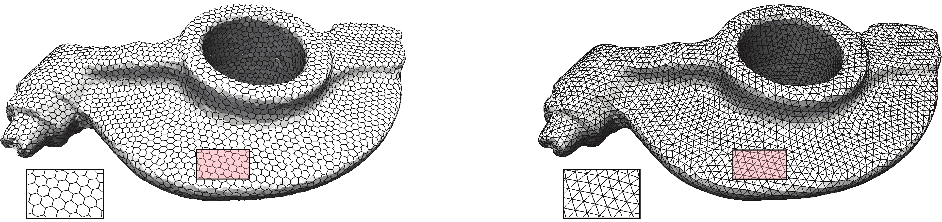
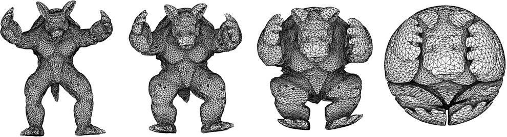
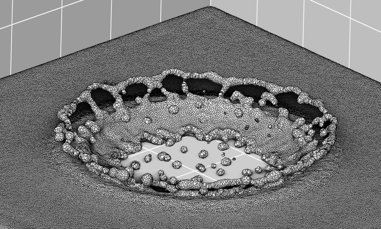
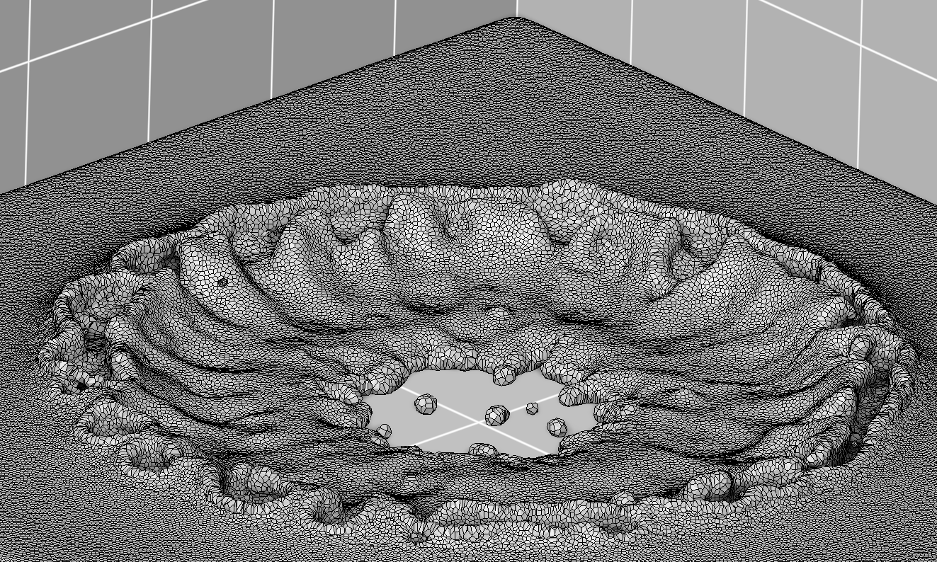
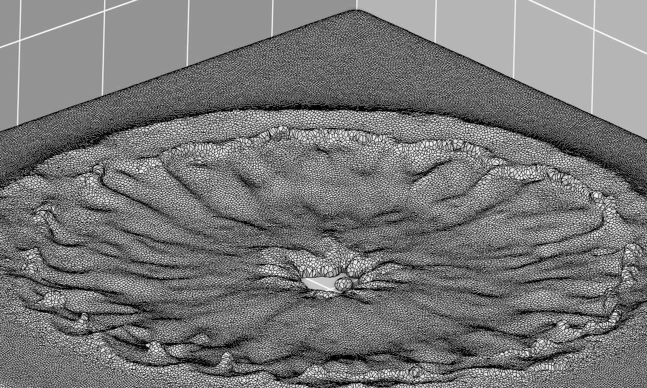
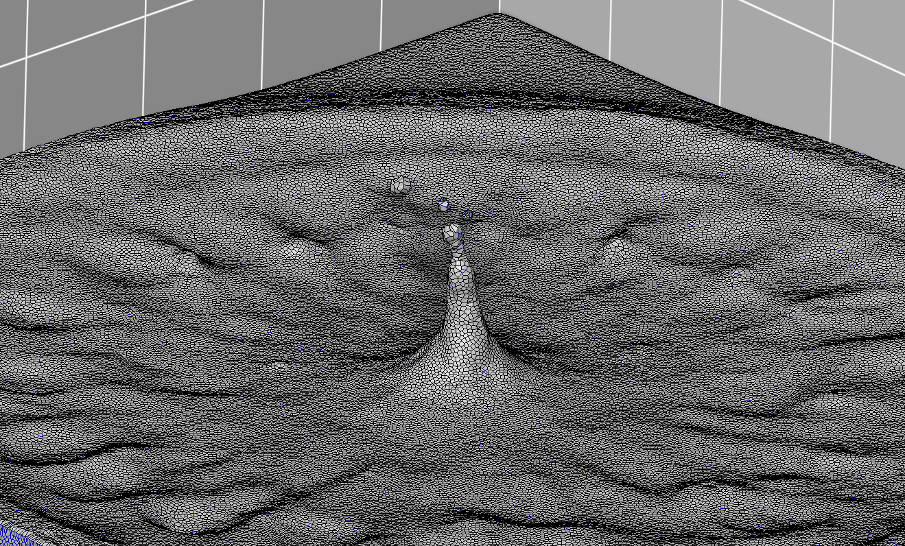
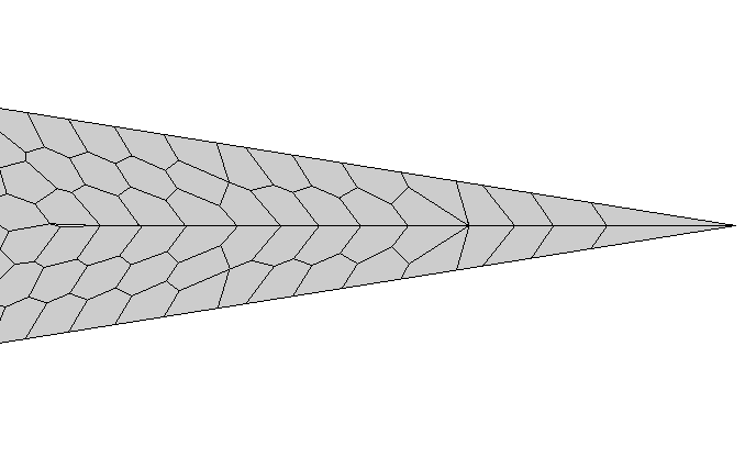
Approximation of displacement interpolation

Sample mesh

Compute transport

Compute barycenters

Compute mesh

Filter triangles

[Lévy 2014]

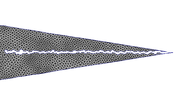
Limits

Meshes play non-symmetric roles
Irregular discontinuities
Erodes original meshes

Introduction to optimal transport
Symmetric semi-discrete optimal transport
Alternating algorithm
Optimization approach
Mesh interpolation
Conclusion

Symmetrization of the semi-discrete transport problem

$(Pow^\phi(x_i))_i$ is an optimal transport plan from $\mu$ to $\sum_i \delta_{x_i}$
$(Pow^\psi(y_i))_i$ is an optimal transport plan from $\nu$ to $\sum_i \delta_{y_i}$

$y_i$ are the barycenters of $Pow^\phi(x_i)$
$x_i$ are the barycenters of $Pow^\psi(y_i)$

Introduction to optimal transport
Symmetric semi-discrete optimal transport
Alternating algorithm
Optimization approach
Mesh interpolation
Conclusion

Alternating algorithm

$x_i$ := random sampling of $\nu$
$y_i$ := random sampling of $\mu$
while not converged do

$(\phi_i)$ := weights of OT from $\mu$ to $(x_i)$
$(y_i)$ := barycenters of $Pow^\phi(x_i)$
$(\psi_i)$ := weights of OT from $\nu$ to $(y_i)$
$(x_i)$ := barycenters of $Pow^\psi(y_i)$

end

Alternating algorithm

$x_i$ := random sampling of $\nu$

$y_i$ := random sampling of $\mu$
while not converged do

$(\phi_i)$ := weights of OT from $\mu$ to $(x_i)$
$(y_i)$ := barycenters of $Pow^\phi(x_i)$
$(\psi_i)$ := weights of OT from $\nu$ to $(y_i)$
$(x_i)$ := barycenters of $Pow^\psi(y_i)$

end

Alternating algorithm

$x_i$ := random sampling of $\nu$

$y_i$ := random sampling of $\mu$

while not converged do

$(\psi_i)$ := weights of OT from $\nu$ to $(y_i)$
$(x_i)$ := barycenters of $Pow^\psi(y_i)$
$(\phi_i)$ := weights of OT from $\mu$ to $(x_i)$
$(y_i)$ := barycenters of $Pow^\phi(x_i)$

end

Alternating algorithm

$x_i$ := random sampling of $\nu$
$y_i$ := random sampling of $\mu$
while not converged do

$(\psi_i)$ := weights of OT from $\nu$ to $(y_i)$

$(x_i)$ := barycenters of $Pow^\psi(y_i)$
$(\phi_i)$ := weights of OT from $\mu$ to $(x_i)$
$(y_i)$ := barycenters of $Pow^\phi(x_i)$

end

Alternating algorithm

$x_i$ := random sampling of $\nu$
$y_i$ := random sampling of $\mu$
while not converged do

$(\psi_i)$ := weights of OT from $\nu$ to $(y_i)$

$(x_i)$ := barycenters of $Pow^\psi(y_i)$

$(\phi_i)$ := weights of OT from $\mu$ to $(x_i)$
$(y_i)$ := barycenters of $Pow^\phi(x_i)$

end

Alternating algorithm

$x_i$ := random sampling of $\nu$
$y_i$ := random sampling of $\mu$
while not converged do

$(\psi_i)$ := weights of OT from $\nu$ to $(y_i)$
$(x_i)$ := barycenters of $Pow^\psi(y_i)$

$(\phi_i)$ := weights of OT from $\mu$ to $(x_i)$

$(y_i)$ := barycenters of $Pow^\phi(x_i)$

end

Alternating algorithm

$x_i$ := random sampling of $\nu$
$y_i$ := random sampling of $\mu$
while not converged do

$(\psi_i)$ := weights of OT from $\nu$ to $(y_i)$
$(x_i)$ := barycenters of $Pow^\psi(y_i)$
$(\phi_i)$ := weights of OT from $\mu$ to $(x_i)$

$(y_i)$ := barycenters of $Pow^\phi(x_i)$

end

Alternating algorithm

$x_i$ := random sampling of $\nu$
$y_i$ := random sampling of $\mu$
while not converged do

$(\psi_i)$ := weights of OT from $\nu$ to $(y_i)$

$(x_i)$ := barycenters of $Pow^\psi(y_i)$
$(\phi_i)$ := weights of OT from $\mu$ to $(x_i)$
$(y_i)$ := barycenters of $Pow^\phi(x_i)$

end

Alternating algorithm

$x_i$ := random sampling of $\nu$
$y_i$ := random sampling of $\mu$
while not converged do

$(\psi_i)$ := weights of OT from $\nu$ to $(y_i)$

$(x_i)$ := barycenters of $Pow^\psi(y_i)$

$(\phi_i)$ := weights of OT from $\mu$ to $(x_i)$
$(y_i)$ := barycenters of $Pow^\phi(x_i)$

end

Alternating algorithm

$x_i$ := random sampling of $\nu$
$y_i$ := random sampling of $\mu$
while not converged do

$(\psi_i)$ := weights of OT from $\nu$ to $(y_i)$
$(x_i)$ := barycenters of $Pow^\psi(y_i)$

$(\phi_i)$ := weights of OT from $\mu$ to $(x_i)$

$(y_i)$ := barycenters of $Pow^\phi(x_i)$

end

Alternating algorithm

$x_i$ := random sampling of $\nu$
$y_i$ := random sampling of $\mu$
while not converged do

$(\psi_i)$ := weights of OT from $\nu$ to $(y_i)$
$(x_i)$ := barycenters of $Pow^\psi(y_i)$
$(\phi_i)$ := weights of OT from $\mu$ to $(x_i)$

$(y_i)$ := barycenters of $Pow^\phi(x_i)$

end

Alternating algorithm

$x_i$ := random sampling of $\nu$
$y_i$ := random sampling of $\mu$
while not converged do

$(\psi_i)$ := weights of OT from $\nu$ to $(y_i)$

$(x_i)$ := barycenters of $Pow^\psi(y_i)$
$(\phi_i)$ := weights of OT from $\mu$ to $(x_i)$
$(y_i)$ := barycenters of $Pow^\phi(x_i)$

end

Alternating algorithm

$x_i$ := random sampling of $\nu$
$y_i$ := random sampling of $\mu$
while not converged do

$(\psi_i)$ := weights of OT from $\nu$ to $(y_i)$

$(x_i)$ := barycenters of $Pow^\psi(y_i)$

$(\phi_i)$ := weights of OT from $\mu$ to $(x_i)$
$(y_i)$ := barycenters of $Pow^\phi(x_i)$

end

Alternating algorithm

$x_i$ := random sampling of $\nu$
$y_i$ := random sampling of $\mu$
while not converged do

$(\psi_i)$ := weights of OT from $\nu$ to $(y_i)$
$(x_i)$ := barycenters of $Pow^\psi(y_i)$

$(\phi_i)$ := weights of OT from $\mu$ to $(x_i)$

$(y_i)$ := barycenters of $Pow^\phi(x_i)$

end

Alternating algorithm

$x_i$ := random sampling of $\nu$
$y_i$ := random sampling of $\mu$
while not converged do

$(\psi_i)$ := weights of OT from $\nu$ to $(y_i)$
$(x_i)$ := barycenters of $Pow^\psi(y_i)$
$(\phi_i)$ := weights of OT from $\mu$ to $(x_i)$

$(y_i)$ := barycenters of $Pow^\phi(x_i)$

end

Alternating algorithm

$x_i$ := random sampling of $\nu$
$y_i$ := random sampling of $\mu$
while not converged do

$(\psi_i)$ := weights of OT from $\nu$ to $(y_i)$
$(x_i)$ := barycenters of $Pow^\psi(y_i)$
$(\phi_i)$ := weights of OT from $\mu$ to $(x_i)$
$(y_i)$ := barycenters of $Pow^\phi(x_i)$

end

Alternating algorithm

$x_i$ := random sampling of $\nu$
$y_i$ := random sampling of $\mu$
while not converged do

$(\psi_i)$ := weights of OT from $\nu$ to $(y_i)$
$(x_i)$ := barycenters of $Pow^\psi(y_i)$
$(\phi_i)$ := weights of OT from $\mu$ to $(x_i)$
$(y_i)$ := barycenters of $Pow^\phi(x_i)$

end

Diagram correspondence

Computation times

Sampling size	Algorithm	Computation time
500	Symmetric	83s
500	Non-symmetric	2s
6500	Non-symmetric	79s

Introduction to optimal transport
Symmetric semi-discrete optimal transport
Alternating algorithm
Optimization approach
Mesh interpolation
Conclusion

Constrained optimization

Lagrangian of the problem: \[\mathcal{L}(X, \Lambda) = F(X) + \Lambda \cdot B(X)\]

where:

$X$ is the vector of parameters
$\Lambda$ is the Lagrange multiplier
$F$ is the sum of transport objective functions
$B$ is the vector of barycentric constraints

Optimality condition

Stationary point $$ \begin{cases} \nabla F(X) + J_B(X)^\top\cdot\Lambda = 0\\ B(X) = 0 \end{cases} $$

Take a step and linearize $$ \begin{cases} \nabla F(X + \delta X) = \nabla F(X) + H_F(X)\delta X + o(\lVert \delta X \rVert)\\ B(X + \delta X) = B(X) + J_B(X)\delta X + o(\lVert \delta X \rVert) \end{cases} $$

Newton’s algorithm

\[ \begin{pmatrix} H_F(X) & J_B(X)^\top\\ J_B(X) & 0 \\ \end{pmatrix} \cdot \begin{pmatrix} \delta X \\ \Lambda \end{pmatrix} = - \begin{pmatrix} \nabla F(X) \\ B(X) \end{pmatrix} \]

Derivatives computation

Reynolds transport theorem [Reynolds 1903]

Optimization results

Computation of second-order derivatives of $F$ and first-order derivatives of $B$
Verified derivatives using finite difference schemes
Does not converge: $(x_i)_i$ and $(\phi_i)_i$ should not be considered independent?

Introduction to optimal transport
Symmetric semi-discrete optimal transport
Alternating algorithm
Optimization approach
Mesh interpolation
Conclusion

Point cloud interpolation

Diagram vertices association

Association of vertices at the intersection of 3 cells

Association of vertices at the intersection of 2 cells and the outside of the mesh

Association of vertices at the intersection of 3 cells splitting during transport

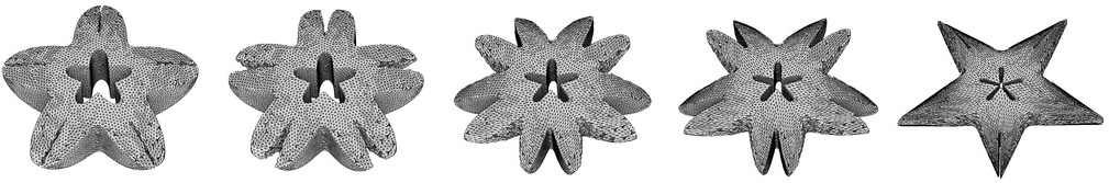
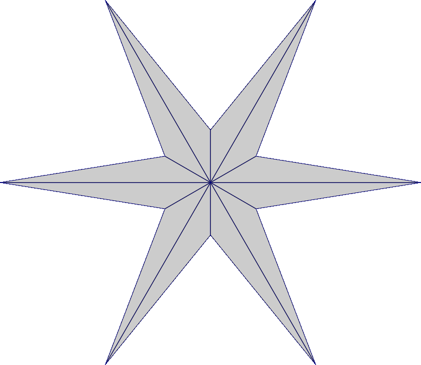
Mesh interpolations

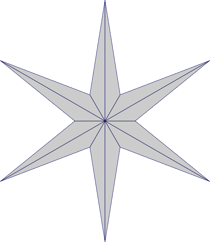$\rightarrow$

Introduction to optimal transport
Symmetric semi-discrete optimal transport
Alternating algorithm
Optimization approach
Mesh interpolation
Conclusion

Conclusion

Symmetrization of the semi-discrete optimal transport problem
Alternating heuristic to compute coupled transport plans
Allows for precise mesh interpolation with relatively few points
Clean capture of discontinuities
Numerically verified derivatives of transport functionals and barycenters constraints

Future work

Proof of convergence
Proof of correspondence between the diagrams
Different optimization method: fulfill barycentric constraints over the space of optimal transport plans

Optimize $\lVert B\rVert$ over the set $$\{(x, \phi, y, \psi) \mid (Pow^\phi(x))\textrm{ and } (Pow^\psi(y)) \textrm{ are optimal transport plans}\}$$

Questions?

Alternating algorithm

More interpolations

Notations

$X = (x_i, \phi_i, y_i, \psi_i)_i \in \mathbb{R}^{6N}$
$Pow^\phi(x_i)$ the cell associated to $x_i$ in the power diagram of sites $(x)$ and weights $(\phi)$
$K_i$ the number of edges of cell $Pow^\phi(x_i)$, $i_k$ the index of its $k$-th neighbor
$\beta_{x,i}(X) = \int_{x\in Pow^\phi(x_i)} (x - y_i)d\mu(x)$ the $i$-th barycentric constraint

Reynolds' transport theorem

Let:

$\Omega(t)$ be an integration domain depending on the real-valued parameter $t$, of boundary $\partial \Omega(t)$
$f(x,t)$ be a function continuous on $\Omega(t)$ and integrable over $\partial \Omega(t)$, of derivative $\frac{\partial f}{\partial t}(x,t)dx$ integrable over $\Omega(t)$
$\gamma(., t) : \mathbb{S}^1 \rightarrow \partial \Omega(t)$ be a parameterization of $\partial \Omega(t)$ defined on the unit circle $\mathbb{S}^1$, so that $\gamma(., t)$ is continuous and piecewise differentiable for all $t$, and $\gamma(\theta, .)$ is $\mathcal{C}^1$ $\forall\theta$
and $n(x)$ is the outwards-pointing normal at $x \in \partial \Omega(t)$

Then the derivative of $\int_{x\in\Omega(t)}f(x, t)dx$ with respect to $t$ is:

Derivative of the centering constraint $\beta_{x,i}$ with respect to the position of the associated site $x_i$

$$\frac{\partial{\beta_{x,i}(X)}_\varepsilon}{\partial x_{i, \eta}} = \sum_{k=1}^{K_i}\frac{1}{\lVert x_i - x_{i_k}\rVert} \int_{x\in E_{i, i_k}} {(x - x_i)}_{\eta}{(x - y_i)}_\varepsilon d\mu(x)$$

Derivative of the centering constraint $\beta_{x,i}$ with respect to the position of a neighboring site $x_{i_k}$

$$\frac{\partial{\beta_{x,i}(X)}_\varepsilon}{\partial x_{i_k, \eta}} = - \frac{1}{\lVert x_{i_k} - x_i}\rVert \int_{x\in E_{i, i_k}}{(x - x_{i_k})}_\eta{(x - y_i)}_\varepsilon d\mu(x)$$

Derivative of the centering constraint $\beta_{x,i}$ with respect to the weight of the associated site $\phi_i$

$$\frac{\partial{\beta_{x,i}(X)}_\varepsilon}{\partial\phi_i}= \sum_{k=1}^{K_i}\frac{1}{2\cdot\lvert x_i - x_{i_k}\rVert} \int_{x\in E_{i, i_k}} {(x - y_i)}_\varepsilon d\mu(x)$$

Derivative of the centering constraint $\beta_{x,i}$ with respect to the weight of a neighboring site $\phi_{i_k}$

$$\frac{\partial{\beta_{x,i}(X)}_\varepsilon}{\partial \phi_{i_k}} = - \frac{1}{2\cdot\lVert x_i - x_{i_k}\rVert} \int_{x\in E_{i, i_k}} {(x - y_i)}_\varepsilon d\mu(x)$$

Derivative of the centering constraint $\beta_{x,i}$ with respect to the \changes{position} of the associated site in the opposite domain $y_i$

$$\frac{\partial {\beta_{x,i}(X)}_\varepsilon}{\partial y_{i, \eta}} = \begin{cases} - \mu(Pow^\phi(x_i)) \text{ if } \varepsilon = \eta \\ 0 \text{ otherwise} \end{cases}$$

Second derivative of $\Phi$ with respect to the same site $x_i$ twice

$$\frac{\partial^2 F(X)}{\partial x_{i, \eta}^2} = 2\cdot\mu(Pow^\phi(x_i)) - 2\cdot \sum_{k=1}^{K_i} \int_{x \in E_{i, i_k}} \frac{{(x_{i, \eta} - x_\eta)}^2}{\lVert x_{i_k} - x_i\rVert} d\mu(x)$$

Second derivative of $\Phi$ with respect to a cell's site $x_i$ and a neighboring site $x_{i_k}$

$$\frac{\partial^2F(X)}{\partial x_{i, \eta}\partial x_{i_k, \eta'}} = 2\cdot \int_{x \in E_{i, i_k}} \frac{{(x_{i_k} - x)}_{\eta'}\cdot{(x_i - x)}_\eta}{\lVert x_{i_k} - x_i\rVert} d\mu(x)$$

Second derivative of $\Phi$ with respect to two different coordinates of the same site $x_i$

$$\frac{\partial^2F(X)}{\partial x_{i, 1} \partial x_{i, 2}}= 2\cdot \sum_{k=1}^{K_i} \int_{x \in E_{i, i_k}} \frac{{(x_i - x)}_1\cdot{(x_i - x)}_2}{\lVert x_{i_k} - x_i\rVert} d\mu(x)$$

Second derivative of $\Phi$ with respect to a site $x_i$ and its corresponding site $y_i$ in the opposite domain

$$\frac{\partial^2F(X)}{\partial x_{i, \eta} \partial y_{i, \eta'}} = 0$$

Second derivative of $\Phi$ with respect to a site $x_i$ and a neighboring site $y_{i_k}$ in the opposite domain

$$ \frac{\partial^2F(X)}{\partial x_{i, \eta} \partial y_{{i_k}, \eta'}} = 0$$

Second derivative of $\Phi$ with respect to the same weight $\phi_i$ twice

$$\frac{\partial F(X)}{\partial \phi_i} = -\sum_{k=1}^{K_i} \frac{1}{2\cdot\lVert x_i - x_{i_k}}\rVert \int_{x\in E_{i, i_k}}d\mu(x)$$

Second derivative of $\Phi$ with respect to a cell's weight $\phi_i$ and the weight $\phi_{i_k}$ of a neighboring cell

$$ \frac{\partial^2F(X)}{\partial\phi_i\partial\phi_{i_k}} = \frac{1}{2\cdot\lVert x_i - x_{i_k}\rVert} \int_{x\in E_{i, i_k}}d\mu(x)$$

Second derivative of $\Phi$ with respect to a cell's weight $\phi_i$ and the weight $\psi_i$ of the corresponding cell in the opposite domain

$$\frac{\partial^2F(X)}{\partial\phi_i\partial\psi_i} = 0$$

Second derivative of $\Phi$ with respect to the weight $\phi_i$ and the site's coordinates $x_i$ of a cell

$$\frac{\partial^2F(X)}{\partial\phi_i\partial x_{i, \eta}} = \sum_{k=1}^{K_i} \frac{1}{\lVert x_i - x_{i_k}\rVert} \int_{x\in E_{i, i_k}} {(x_i - x)}_\eta d\mu(x)$$

Second derivative with respect to the weight $\phi_i$ of a cell and the coordinates $x_{i_k}$ of a neighboring cell's site

$$\frac{\partial^2F(X)}{\partial\phi_i\partial x_{i_k, \eta}} = -\frac{1}{\lVert x_i - x_{i_k}\rVert} \int_{x\in E_{i, i_k}} {(x_{i_k} - x)}_\eta d\mu(x)$$

Second derivative with respect to the weight $\phi_i$ of a cell and the coordinates $y_i$ of the corresponding site in the opposite domain

$$\frac{\partial^2 F(X)}{\partial \phi_i\partial y_{i, \eta}} = 0$$

Inverting the constraints and the objective function

Optimize $\lVert B\rVert$ over the set $\{(x, \phi, y, \psi) \mid (Pow^\phi(x))\textrm{ and } (Pow^\psi(y)) \textrm{ are optimal transport plans}\}$
Optimizing over the set of optimal transport plans: the value of $(x)$ determines the optimal weights $\phi^*(x)$
Cancel $B(x, \phi^*(x), y, \psi^*(y))$ using Newton's method or minimize $\lVert B(x, \phi^*(x), y, \psi^*(y)) \rVert$.
Parameter set is reduced to $(x, y)$.